proBatch: Tools for Diagnostics and Corrections of Batch Effects in Proteomics
proBatch简介 proBatch是便于在高通量实验中进行批量效应分析和校正的分析工具。主要为质谱蛋白质组学(DIA/SWATH)开发,但也可在调整后应用于大多数的Omic数据。
诊断(蛋白质组/基因组范围和特征水平)
校正(归一化和批次效应校正)
基于非线性拟合的方法来处理复杂的、质谱特有的信号漂移
质量控制
安装 安装所需的其它包 proBatch主要通过调用其它包中的函数实现功能,因此依赖于许多其它已有的R包。如果其中一些包未安装,则需要在运行proBatch之前安装。
1
2
3
4
5
6
bioc_deps <- c ("GO.db" , "impute" , "preprocessCore" , "pvca" ,"sva" ) cran_deps <- c ("corrplot" , "data.table" , "ggplot2" , "ggfortify" ,"lazyeval" , "lubridate" , "pheatmap" , "reshape2" ,"readr" , "rlang" , "tibble" , "dplyr" , "tidyr" , "wesanderson" ,"WGCNA" ) if (!requireNamespace("BiocManager" , quietly = TRUE )) install.packages("BiocManager" ) BiocManager::install(bioc_deps) install.packages(cran_deps)
安装proBatch 可通过以下三个途径获取proBatch包:
1
2
3
4
if (!requireNamespace("BiocManager" , quietly = TRUE )) install.packages("BiocManager" ) BiocManager::install("proBatch" )
1
2
library(devtools) install_github("symbioticMe/proBatch" , build_vignettes = TRUE )
proBatch的使用 要查看与系统中安装的proBatch版本相对应的说明文档,启动R并输入:
1 browseVignettes("proBatch" )
使用前的tips
一些基本的数据处理步骤已经完成,如已经完成搜库比对、FDR control、log-transformation等
数据过滤。应过滤掉诱饵测量值(decoy measurements)以确保正确的样本强度分布对齐。过滤掉低质量的样本(通常通过鉴定肽的总强度或样品的相关性来确定)
建议在批次效应校正之前不要填补缺失值
在消除批次效应之后再进行蛋白质定量
Preparing for data analysis Loading the libraries 加载所需的包,以便后续步骤的使用。
1
2
3
4
require(dplyr) require(tibble) require(ggplot2) library(proBatch)
数据分析需要三个数据表,即:
measurement (data matrix)
sample annotation
feature annotation (optional) tables
如果对BioBase数据比较熟悉,则可认为上述的三种数据是:
assayData
joined phenoData and protocolData
featureData
三种数据可参考包中给出的示例数据
1 data('example_proteome' , 'example_sample_annotation' , 'example_peptide_annotation' , package = 'proBatch' )
或proBatch overview 中的详细说明。
其它有用的函数 1 2 3 4 5 6 7 example_matrix <- long_to_matrix(example_proteome, feature_id_col = 'peptide_group_label' , measure_col = 'Intensity' , sample_id_col = 'FullRunName' ) log_transformed_matrix <- log_transform_dm(example_matrix, log_base = 2 , offset = 1 ) color_list <- sample_annotation_to_colors(example_sample_annotation, factor_columns = c ('MS_batch' , 'digestion_batch' , 'EarTag' , 'Strain' , 'Diet' , 'Sex' ), numeric_columns = c ('DateTime' ,'order' ))
Initial assessment of the raw data matrix Plotting the sample mean proBatch建议在处理批次效应之后再填补缺失值,但包中没有兼容存在缺失值的情况,如果有缺失值无法计算mean。plot_sample_mean函数主要实现的功能为计算样本均值并绘制样本均值散点图,横坐标为样本顺序(order),纵坐标为样本均值(Mean_Intensity),并以不同颜色表示样本的batch。可通过自行编写能够兼容缺失值的代码实现这一功能。
1 2 3 4 5 6 7 8 9 10 plot_sample <- data.frame(row.names = colnames(log_transformed_matrix)) colnum <- ncol(log_transformed_matrix) for (i in c (1 :colnum)){ item <- colnames(log_transformed_matrix)[i] plot_sample[item, "mean" ] <- mean(log_transformed_matrix[,i], na.rm=T ) plot_sample[item,"MS_batch" ] <- sample_anno[i,"MS_batch" ] plot_sample[item,"order" ] <- sample_anno[i,"order" ] } ggplot(plot_sample, aes(order, mean, color = MS_batch)) + geom_point() + xlab("order" ) + ylab("Mean_intensity" ) + ylim(0 ,15 )
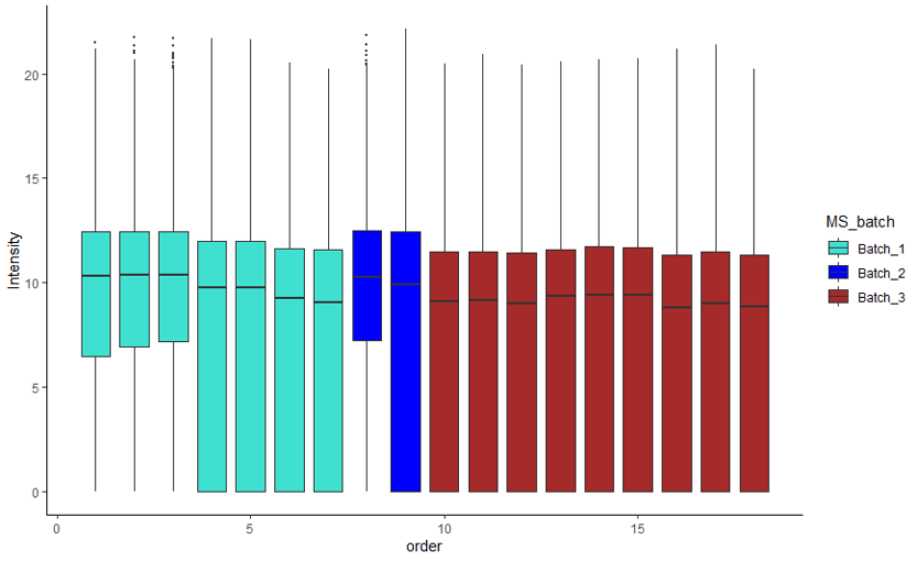
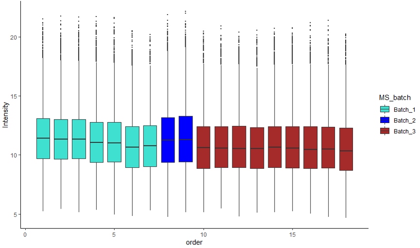
Plotting boxplots 绘制箱图观察数据:
1 2 3 log_transformed_long <- matrix_to_long(log_transformed_matrix) batch_col = 'MS_batch' plot_boxplot(log_transformed_long, example_sample_annotation, batch_col = batch_col, color_scheme = color_list[[batch_col]])
利用PEAKS数据做到这一步时发现产生的箱图向0偏,即含有大量0值。这是PEAKS搜库结果的一个特点,除了缺失值还会有大量intensity被定量为0。在之前处理PEAKS数据时,log-transformation步骤会将0转换为NA,在后续步骤也当作缺失值处理。log_transform_dm会将0保留为0,导致使用PEAKS数据画箱图时出现问题。返回log-transformation步骤使用自己写的处理代码处理数据后,箱图绘制与预期一致。
Normalization 包中提供Median Normalization和Quantiles Normalization,可直接使用。
1 2 3 4 5 6 7 8 median_normalized_matrix = normalize_data_dm(log_transformed_matrix, normalize_func = 'medianCentering' ) median_normalized_matrix = normalize_data_dm(example_matrix, normalize_func = 'medianCentering' , log_base = 2 , offset = 1 ) quantile_normalized_matrix = normalize_data_dm(log_transformed_matrix, normalize_func = 'quantile' )
后续相应的画图观察处理后的数据时,应注意Inf值的影响。数据中如有Inf或-Inf,可通过data[data == Inf] <- NA或data[data == -Inf] <- NA将其替换。Inf出现是因为在log转换时没有处理好0值。
Diagnostics of batch effects in normalized data Hierarchical clustering & heatmap 1 2 3 4 5 selected_annotations <- c ('MS_batch' , 'digestion_batch' , 'Diet' ) plot_hierarchical_clustering(quantile_normalized_matrix, sample_annotation = example_sample_annotation, color_list = color_list, factors_to_plot = selected_annotations, distance = 'euclidean' , agglomeration = 'complete' , label_samples = FALSE ) plot_heatmap_diagnostic(quantile_normalized_matrix, example_sample_annotation, factors_to_plot = selected_annotations, cluster_cols = TRUE , color_list = color_list, show_rownames = FALSE , show_colnames = FALSE )
根据报错信息可知color_list一项一直与我的数据不兼容,因此注释行显示不完全。
PCA & PVCA PCA和PVCA使用时,缺失值会被直接填为-1。
1 2 3 4 5 6 7 8 9 10 11 12 13 pca1 = plot_PCA(median_normalized_matrix, sample_anno, color_by = 'MS_batch' , plot_title = 'MS batch' , color_scheme = color_list[['MS_batch' ]]) pca2 = plot_PCA(median_normalized_matrix, sample_anno, color_by = 'digestion_batch' , plot_title = 'Digestion batch' , color_scheme = color_list[['digestion_batch' ]]) pca3 = plot_PCA(median_normalized_matrix, sample_anno, color_by = 'order' , plot_title = 'order' , color_scheme = color_list[['order' ]]) pca4 = plot_PCA(median_normalized_matrix, sample_anno, color_by = 'DateTime' , plot_title = 'DateTime' , color_scheme = color_list[['DateTime' ]]) library(ggpubr) ggarrange(pca1, pca2, pca3, pca4, ncol = 2 , nrow = 2 ) technical_factors = c ('MS_batch' , 'digestion_batch' ) biological_factors = NULL biospecimen_id_col = 'EarTag' plot_PVCA(median_normalized_matrix, sample_anno, technical_factors = technical_factors, biological_factors = biological_factors)
Peptide-level diagnostics and spike-ins 这一步骤需要将来自同一蛋白的肽段注释在一起。如果缺少肽段的注释信息,这一步骤无法正常进行。
1 2 median_normalized_long <- matrix_to_long(median_normalized_matrix) plot_spike_in(median_normalized_long, sample_anno, peptide_annotation = peptide_anno, protein_col = 'Gene' , spike_ins = 'BOVINE_A1ag' , plot_title = 'Spike-in BOVINE protein peptides' , color_by_batch = TRUE , color_scheme = color_list[[batch_col]])
correction batch effect Continuous drift correction 处理连续型批次效应使用LOESS拟合。
1 2 3 loess_fit_df <- adjust_batch_trend_df(quantile_normalized_long, example_sample_annotation) loess_fit_70 <- adjust_batch_trend_df(median_normalized_long, sample_anno, span = 0.7 ) plot_with_fitting_curve(feature_name = 'N(+.98)NATVHEQVGGPSLTSDLQAQSK' , fit_df = loess_fit_70, fit_value_col = 'fit' , df_long = median_normalized_long, sample_annotation = sample_anno, color_by_batch = TRUE , color_scheme = color_list[[batch_col]], plot_title = 'Span = 70%' )
Discrete batch correction 处理离散型批次效应可通过median centering (per feature per batch)和ComBat进行。
1 2 3 4 5 6 7 peptide_median_df <- center_feature_batch_medians_df(loess_fit_df, sample_anno) plot_single_feature(feature_name = 'N(+.98)NATVHEQVGGPSLTSDLQAQSK' , df_long = peptide_median_df, sample_annotation = sample_anno, measure_col = 'Intensity' , plot_title = 'Feature-level Median Centered' ) comBat_df <- correct_with_ComBat_df(loess_fit_df, example_sample_annotation) plot_single_feature(feature_name = '10231_QDVDVWLWQQEGSSK_2' , df_long = loess_fit_df, sample_annotation = example_sample_annotation, plot_title = 'Loess Fitted' )
Correct batch effects: universal function proBatch提供一个方便的多合一的函数来进行批量校正。correct_batch_effects_df()能在一次函数调用中可修正MS信号漂移和离散位移。只需在discrete_func中指定首选的离散校正方法,即"ComBat "或 "MedianCentering"。并补充其他参数,如adjust_batch_trend_df()中的span、abs_threshold或pct_threshold。
1 2 batch_corrected_df <- correct_batch_effects_df(df_long = median_normalized_long, sample_annotation = sample_anno,discrete_func = 'ComBat' ,continuous_func = 'loess_regression' ,abs_threshold = 5 , pct_threshold = 0.20 ) batch_corrected_matrix <- long_to_matrix(batch_corrected_df)
Quality control Heatmap of selected replicate samples 挑选重复组计算相关性并绘制热图观察批次效应处理结果。
1 2 3 4 5 6 7 8 9 10 11 12 13 14 15 16 17 earTags <- c ('ET1524' , 'ET2078' , 'ET1322' , 'ET1566' , 'ET1354' , 'ET1420' , 'ET2154' , 'ET1515' , 'ET1506' , 'ET2577' , 'ET1681' , 'ET1585' , 'ET1518' , 'ET1906' ) replicate_filenames = example_sample_annotation %>% filter(MS_batch %in% c ('Batch_2' , 'Batch_3' )) %>% filter(EarTag %in% earTags) %>% pull(!!sym('FullRunName' )) p1_exp = plot_sample_corr_heatmap(log_transformed_matrix, samples_to_plot = replicate_filenames, plot_title = 'Correlation of selected samples' ) breaksList <- seq(0.7 , 1 , by = 0.01 ) heatmap_colors = colorRampPalette(rev(RColorBrewer::brewer.pal(n = 7 , name = 'RdYlBu' )))(length (breaksList) + 1 ) factors_to_show = c (batch_col, biospecimen_id_col) p1 = plot_sample_corr_heatmap(log_transformed_matrix, samples_to_plot = replicate_filenames,sample_annotation = example_sample_annotation, factors_to_plot = factors_to_show, plot_title = 'Log transformed correlation matrix of selected replicated samples' , color_list = color_list, heatmap_color = heatmap_colors, breaks = breaksList, cluster_rows= FALSE , cluster_cols=FALSE ,fontsize = 4 , annotation_names_col = TRUE , annotation_legend = FALSE , show_colnames = FALSE ) p2 = plot_sample_corr_heatmap(batch_corrected_matrix, samples_to_plot = replicate_filenames, sample_annotation = example_sample_annotation, factors_to_plot = factors_to_show, plot_title = 'Batch Corrected selected replicated samples' , color_list = color_list, heatmap_color = heatmap_colors, breaks = breaksList, cluster_rows= FALSE , cluster_cols=FALSE ,fontsize = 4 , annotation_names_col = TRUE , annotation_legend = FALSE , show_colnames = FALSE ) library(gridExtra) grid.arrange(grobs = list (p1$gtable, p2$gtable), ncol=2 )
由于缺失值的存在,直接使用包中函数进行这一步骤失败,自己写代码代替。
1 2 3 4 5 library(pheatmap) mcor <- cor(select_replicate_samples, method = 'pearson' , use = "complete.obs" ) pheatmap(mcor, cellwidth = 25 , cellheight = 25 , color = colorRampPalette(c ("#ffffff" , "#4682b4" ))(100 ))
Correlation distribution of samples 绘制相同或不同批次的生物重复和非生物重复之间的相关分布。
1 2 3 4 5 6 7 8 9 10 sample_cor_raw <- plot_sample_corr_distribution(log_transformed_matrix, example_sample_annotation,repeated_samples = replicate_filenames, batch_col = 'MS_batch' , biospecimen_id_col = 'EarTag' , plot_title = 'Correlation of samples (raw)' , plot_param = 'batch_replicate' ) raw_corr = sample_cor_raw + theme(axis.text.x = element_text(angle = 45 , hjust = 1 )) + ylim(0.7 ,1 ) + xlab(NULL ) sample_cor_batchCor <- plot_sample_corr_distribution(batch_corrected_matrix, example_sample_annotation, batch_col = 'MS_batch' , plot_title = 'Batch corrected' , plot_param = 'batch_replicate' ) corr_corr = sample_cor_batchCor + theme(axis.text.x = element_text(angle = 45 , hjust = 1 )) + ylim(0.7 , 1 ) + xlab(NULL ) library(gtable) library(grid) g2 <- ggplotGrob(raw_corr) g3 <- ggplotGrob(corr_corr) g <- cbind(g2, g3, size = 'first' ) grid.draw(g)
Correlation of peptide distributions within and between proteins 来自同一蛋白的肽段之间会有更强的相关性,通过计算蛋白内和蛋白间肽段的相关性观察批次效应处理结果。
1 2 3 4 5 6 peptide_cor_raw <- plot_peptide_corr_distribution(log_transformed_matrix, example_peptide_annotation, protein_col = 'Gene' , plot_title = 'Peptide correlation (raw)' ) peptide_cor_batchCor <- plot_peptide_corr_distribution(batch_corrected_matrix, example_peptide_annotation, protein_col = 'Gene' , plot_title = 'Peptide correlation (batch correcte)' ) g2 <- ggplotGrob(peptide_cor_raw+ ylim(c (-1 , 1 ))) g3 <- ggplotGrob(peptide_cor_batchCor+ ylim(c (-1 , 1 ))) g <- cbind(g2, g3, size = 'first' ) grid.draw(g)
参考 [1] proBatch Manual proBatch Overview